Simulate 13C breath time series data

Generates simulated breath test data, optionally with errors. If none of the three standard deviations m_std, k_std, beta_std is given, an empirical covariance matrix from USZ breath test data is used. If any of the standard deviations is given, default values for the others will be used.

Usage

simulate_breathtest_data(
  n_records = 10,
  m_mean = 40,
  m_std = NULL,
  k_mean = 0.01,
  k_std = NULL,
  beta_mean = 2,
  beta_std = NULL,
  noise = 1,
  cov = NULL,
  student_t_df = NULL,
  missing = 0,
  seed = NULL,
  dose = 100,
  first_minute = 5,
  step_minute = 15,
  max_minute = 155
)

Arguments

n_records

Number of records

m_mean, m_std

Mean and between-record standard deviation of parameter m giving metabolized fraction.

k_mean, k_std

Mean and between-record standard deviation of parameter k, in units of 1/minutes.

beta_mean, beta_std

Mean and between-record standard deviations of lag parameter beta

noise

Standard deviation of normal noise when student_t_df = NULL; scaling of noise when student_t_df >= 2.

cov

Covariance matrix, default NULL, i.e. not used. If given, overrides standard deviation settings.

student_t_df

When NULL (default), Gaussian noise is added; when >= 2, Student_t distributed noise is added, which generates more realistic outliers. Values from 2 to 5 are useful, when higher values are used the result comes close to that of Gaussian noise. Values below 2 are truncated to 2.

missing

When 0 (default), all curves have the same number of data points. When > 0, this is the fraction of points that were removed randomly to simulate missing

seed

Optional seed; not set if seed = NULL (default)

dose

Octanoate/acetate dose, almost always 100 mg, which is also the default

first_minute

First sampling time. Do not use 0 here, some algorithms do not converge when data near 0 are passed.

step_minute

Inter-sample interval for breath test

max_minute

Maximal time in minutes.

Value

A list of class simulated_breathtest_data with 2 elements:

record

Data frame with columns patient_id(chr), m, k, beta, t50 giving the effective parameters for the individual patient record.

data

Data frame with columns patient_id(chr), minute(dbl), pdr(dbl) giving the time series and grouping parameters.

A comment is attached to the return value that can be used as a title for plotting.

Examples

library(ggplot2)
pdr = simulate_breathtest_data(n_records = 4, seed = 4711, missing = 0.3,
       student_t_df = 2, noise = 1.5) # Strong outliers
#
str(pdr, 1)  
#> List of 2
#>  $ record:'data.frame':	4 obs. of  5 variables:
#>   ..- attr(*, "cov")= num [1:3, 1:3] 1.88e+02 -2.60e-02 -2.04 -2.60e-02 7.74e-06 4.77e-04 -2.04 4.77e-04 1.82e-01
#>   .. ..- attr(*, "dimnames")=List of 2
#>  $ data  : tibble [31 × 3] (S3: tbl_df/tbl/data.frame)
#>   ..- attr(*, "comment")= chr "4 records,  m = 40, k =  0.010, beta =  2.0, cov-matrix, \n Student-t 2 df noise amplitude = 2, 30% missing"
#>  - attr(*, "class")= chr [1:2] "simulated_breathtest_data" "list"
#
pdr$record # The "correct" parameters
#>   patient_id  m      k beta t50_maes_ghoos
#> 1     rec_01 30 0.0086  2.0            142
#> 2     rec_02 27 0.0140  2.4            100
#> 3     rec_03 46 0.0098  1.4             97
#> 4     rec_04 56 0.0076  2.2            169
#
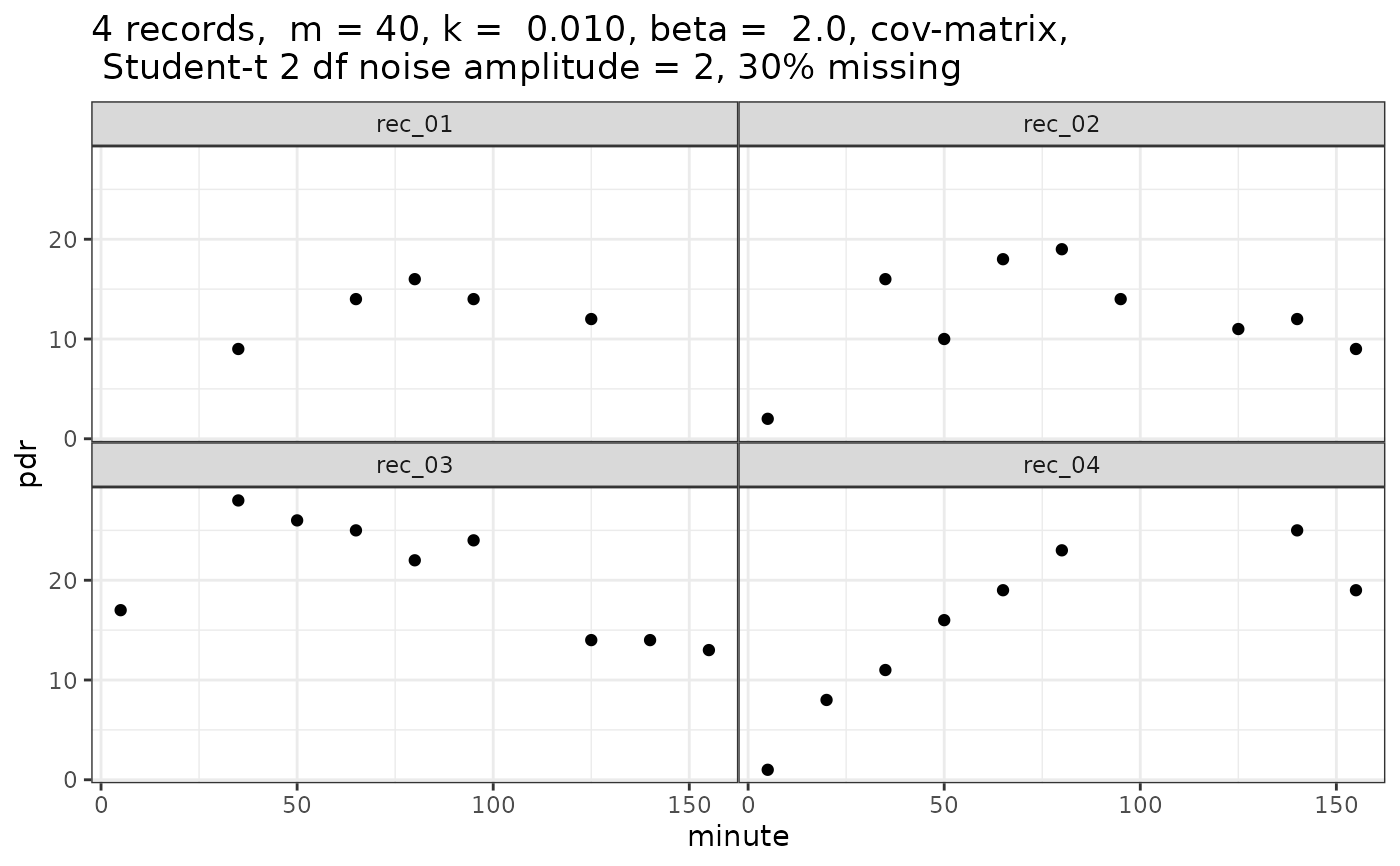
# Explicit plotting
ggplot(pdr$data, aes(x = minute, y = pdr)) + geom_point() +
  facet_wrap(~patient_id) + ggtitle(comment(pdr$data))

#
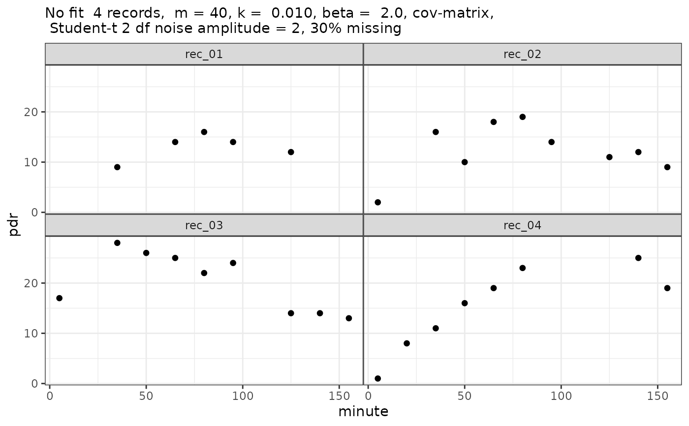
# Or use cleanup_data and null_fit for S3 plotting
plot(null_fit(cleanup_data(pdr$data)))