Methods and concepts

Dieter Menne, Menne Biomed Consulting Tuebingen, dieter.menne@menne-biomed.de

A heretical view on ¹³C breath test for gastric emptying

¹³C breath test data are evaluated in clinical practice and in research as an indirect measure of gastric emptying. The normative literature on the underlying concepts is given in the documentation of exp_beta(), t50_maes_ghoos() and t50_bluck_coward().

Here, I present a subjective viewpoint on the pharmakokinetics of breath test time series. After a look at the Maes/Ghoos method (Ghoos et al. (1993), Maes et al. (1998)) as it is currently used, alternatives are discussed in the next section.

Current concepts

Within the standard framework implemented in this package, data are fitted to an exponential beta function

\[{PDR} = m*{dose}*k*\beta(1-e^{-k*minute})^{(\beta - 1)}*e^{-k*minute}\]

Written in R code

exp_beta = function(minute,dose,m,k,beta) {
     m*dose*k*beta*(1-exp(-k*minute))^(beta-1)*exp(-k*minute)
}

The figure below shows examples of emptying curves. The so-called lag time of the Maes/Ghoos method is at the time of the maximum. Calling this “lag” is a highly confusing definition; technically, lag is the time until a first noticeable rise occurs in the curve, best illustrated by the blue curves with beta = 8, which has an estimated lag of about 15 minutes. If one looks more closely, even this definition is misleading, because the curves with higher beta are not zero, but behave like a polynomial curve with a power of beta - 1 at the origin. A real lag would be best illustrated by a curve shifted to the right by t_lag and pdr values of 0 for t < t_lag, indicating a real physical transport of the meal from the stomach to the small intestine.

In practice, when ¹³C curves are fitted, beta is typically in the range of 1.5 and 2.5; values of beta near 1 often lead to instabilities and are protected by priors in the Bayesian breathteststan::stan_fit() implemented in package breathteststan.

Warning: 
[1m
[22mUsing `size` aesthetic for lines was deprecated in ggplot2 3.4.0.

[36mℹ
[39m Please use `linewidth` instead.

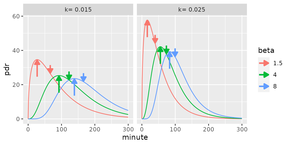
Examples of exponential beta functions used to fit breath test curves. Bottom-up arrow: Maes/Ghoos lag time. Top-down arrow: Maes/Ghoos half emptying time.

The half-emptying as defined by Maes et al. (1998) is the time where the area under curve (AUC) is half the AUC extrapolated to infinity. In pharmakokinetics terms, it is the time where half of the bioavailable ¹³C has been metabolized. This time is determined both by gastric emptying and by the pharmacokinetics of ¹³C bound in octanoate/acetate.

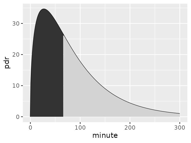
The half-emptying time in the definition of Maes/Ghoos is the time where the area under curve (AUC) is half of the AUC under the curve extrapolated to infinity.

The AUC extrapolated to infinity, which is the denominator in the definition of t50, is a vulnerable variable. Even if we accept that the exponential beta function is a reasonable model for breath test time series, extrapolating individual curves from data only slightly longer than t50 results in ambiguous area estimates, often fails to converge, and even more often gives wildly romantic estimates of t50.

To illustrate how brittle the AUC to infinity is, look back at a different function that had been used to fit ¹³C time series. Ghoos et al. (1993) used the following Gamma function to fit the data:

\[pdr = a*t^b*e^{-ct}\] As the figure below shows, this function gives perfectly valid fits of breath test time series. However, the area under curve extrapolated to infinity is infinite, so it cannot be used to compute a half-emptying time from the AUC.

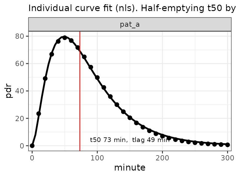
Gamma function from Ghoos et al. (1993) definition as points, and fitted beta exponential as line. Both function look very similar, but the area under the gamma function is infinite and thus cannot be used to compute t50.

Dieter’s soapbox

I therefore recommend using one of the population method, as implemented in nlme_fit() and stan_fit() for studies; these methods provide “borrowing strength” to keep the flock of lambs safely together and protect outliers from the big bad wolf.

• If you write or review a paper that uses single curve fits to report study results, rewrite or reject it. Using the function provided in this package is free as in beer and in speech, and when you use the online version, you do not even have to install R. The vignette gives details on how to prepare your data with Excel.
• For clinical practice, you have single measurements for which you want an immediate result. You can use the Bayesian method to get regularized estimates; or, if you want to be fancy, prepare a data set of some of your previous cases, add the new patient’s data as a mix-in, and use the Mixed-model or the Bayesian fit.

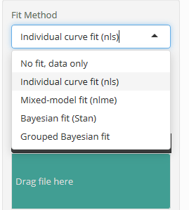
The fitting methods available in package breathtestshiny and in the online version.

A second look

The half-emptying time determined with the ¹³C breath test method correlates to some extend with gastric emptying in within-subject measurements, but it is not more than a surrogate for gastric emptying times measured by MRI (with secretion) or scintigraphy (meal-only). For data set usz_13c_d in this package, MRI emptying data are available and can be compared with breath test data. The type of meal strongly biases the estimates because of the the dependency on lipophilic/lipophobic layering; comparing different meal types is not reliable even within-subject, and less so between-subject.

Many attempts have been made to extract more information from the emptying curve, and to correct for the overall too high values; the Bluck-Coward method implemented in this package is one of them, but the results are are even less consistent with those from MRI than those from the Maes/Ghoos method. Sanaka et al. (2004) mention deconvolution and use an approximate correction for the pharmcological weighting function for the Wagner-Nelson method.

There are many publication that tried an ad-hoc scintigraphic correction (Keller et al. (2009), t50_maes_ghoos_scintigraphy()) or one based on pharmacolokinetics (Bluck and Coward (2006), t50_bluck_coward()). I do not know of any publication which has used rigorous statistical tests such as statistical cross-validation and validation with different meal types to show that some method gives “better” results than the default Maes/Ghoos method.

In the following, I argue that there is nothing to gain from playing with “better” methods to fit the breath test time series. Independent per-subject information must be available to separate acetate pharmacokinetics, based on concentration gradient diffusion, from gastric empyting, which is physical transport.

Acetate pharmacology

Assume we do not mix the labelled acetate with the meal, but hide it in acid-resistant coating as it is used for PPI tablets. No ¹³C will be recorded as long as the tablet is in the stomach, but it will quickly release ¹³C labelled acetate in the duodenum or small intestine, mimicing a one-time dose. As described by standard pharmacokinetics, this results in a PDR response following a first-order compartmental model. Forgetting about decorative normalization constants, the response is the difference between two exponential functions:

\[{foc} = e^{-k_1 * {minute}} - e^{-k_2 * {minute}}\] The normalization constant includes clearance and dose and only scales the curve. The correct normalization constants can be found in standard texts on pharmacokinetics (Gabrielsson and Weiner (2006)) or in as a base R function stats::SSfol() in Pinheiro and Bates (2000).

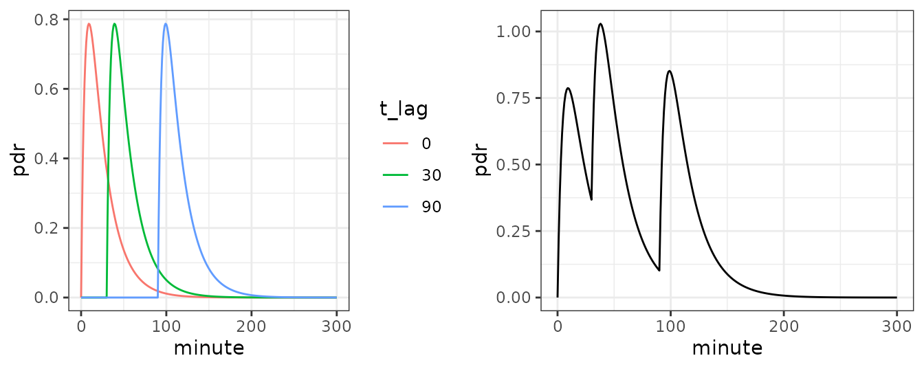
Left: pharmcological PDR response of separated loads released in the smaller bowel after 0, 30 and 90 minutes. Right: sum response when all three loads are released successively.

The left panel in the above plot shows three examples of ¹³C fed by an enteric tables, remaining in the stomach for 0, 30 and 90 minutes and then quickly being released in the smaller intestine. Note that we have a real lag caused by physical transport here: before the tablet is in the smaller bowel, there is no response at all. This is different from the polynomial-like pseudo-lag with the beta-exponential function.

The right panel in the above plot shows the summary PDR curve when the three tablets are fed together and by chance are released after 0, 30 and 90 minutes. This mimics the case of a stomach releasing the meal in three chunks of the same size and composition, well known from pharmacokinetics for multiple doses of a drug.

The real flow out of the stomach is not pulse-like, but more like that of a continuous infusion with changing flow. When we assume that the stomach empties with a power-exponential function as in the left panel (see gastempt::powexp()), the flow is a wide peak as shown in the right panel below. The PDR response technically is the convolution of the flow with the pulse response shown as red curve (t_lag = 0) in the above plot.

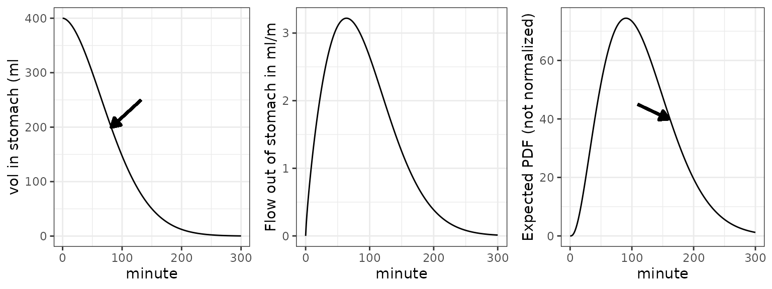
Meal volume (left) and flow when gastric emptying function is a power exponential function. Slope was computed with function gastempt::powexp_slope() with inverted sign. 400 ml initial value, tempt = 100, beta = 1.8 Half empyting times t50 are marked by arrows.

The correct half-emptying time t50 in this example was 82 minutes, as determined from the left panel; t50 determined by fitting with the Maes/Ghoos version in the right panel was 109 minutes.

The bias from fitting the PDR curve naively is caused by the convolution of mechanical transport in gastric emptying, and pharmacological drug kinetics. The latter is a nuisance parameter and should be eliminated - or is it a parameter of interest in its own?

How to correct for the pharmacological bias?

I propose a revised procedure to separate pharmacology from transport. Patient first receive 30 mg acetate in an enteric table together with water. DOB data are recorded for 60 minutes, and after that the normal procedure of meal with 100 mg acetate/octanoate. The resulting PDR will look as follows:

  data.frame(pdr = c(ff_0[0:59]*50, rep(0, 20), cv$pdr)) %>% 
  mutate(
    minute = 0:(n()-1)
  ) %>% 
  filter(minute %% 10 == 0) %>% 
  mutate(
    pdr = pdr + rnorm(n(), 0, 1)
  ) %>% 
  ggplot(aes(x = minute, y = pdr)) +
           geom_point() + geom_line(col = "gray") +
  scale_x_continuous(breaks = seq(0, 360, by = 60))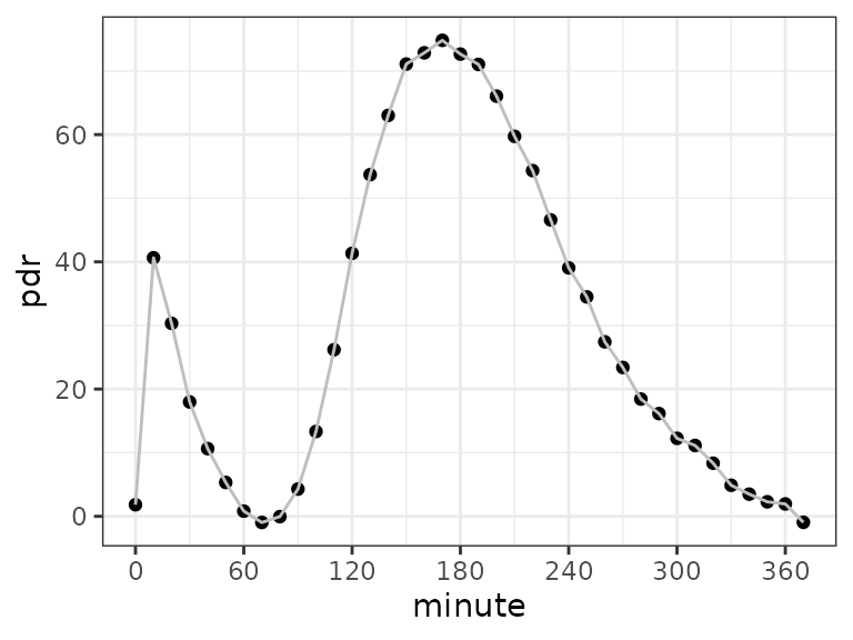

Simulated response of a two-stage breath test procedure. The peak within the first hour is from acetate directly released in the small bowel, the second wider peak is the result of the convolution of transport emptying and pharmacokinetics.

The first narrow peak up to 1 hour is the pharmacological response; by fitting it, the kinetic time constants that broaden the wide peak can be determined, and can be used to remove the bias of the transport component visible in the main peak by mathematical deconvolution.

Can anyone supply a data set for a pilot?

Why do we need population fits?

Why no Wagner-Nelson (Sanaka)?

A popular alternative when curve fitting does not work was the Wagner-Nelson (Sanaka et al. (2004)) method which uses a non-parametric approach for the initial slope. However, it uses the assumption that the terminal slope is the same for all subjects (k=0.01/min, 0.65/h) which strongly affects the estimate of the half-emptying time, so there is little justification to use the Wagner-Nelson method.

With some of the functions in this package or with breathteststan::stan_fit() in the sister package, all curves can be fitted. I have not seen a single example that fails with the Bayesian method when multiple records are analyzed with a mix-in, so there is no excuse to use the Wagner-Nelson method any longer.

If you must, you can use function ComputeAndSaveWNFit in my legacy package D13CBreath. The function is somewhat awkward to use because it has been written for an application with a tightly integrated database, but feel free to steal the code and run.

Citations

Bluck, Leslie J C., and W Andy Coward. 2006. “Measurement of Gastric Emptying by the 13C-Octanoate Breath Test–Rationalization with Scintigraphy.” Physiol Meas 27 (3): 279–89. https://doi.org/10.1088/0967-3334/27/3/006.

Gabrielsson, Johan, and Dan Weiner. 2006. Pharmacokinetic & Pharmacodynamic Data Analysis : Concepts and Applications. 4. ed., rev. and expanded. Stockholm: Swedish Pharmaceutical Press.

Ghoos, Y. F., B. D. Maes, B. J. Geypens, G. Mys, M. I. Hiele, P. J. Rutgeerts, and G. Vantrappen. 1993. “Measurement of Gastric Emptying Rate of Solids by Means of a Carbon-Labeled Octanoic Acid Breath Test.” Gastroenterology 104 (6): 1640–47. https://doi.org/10.1016/0016-5085(93)90640-x.

Keller, J, V Andresen, J Wolter, P Layer, and M Camilleri. 2009. “Influence of Clinical Parameters on the Results of 13C-Octanoic Acid Breath Tests: Examination of Different Mathematical Models in a Large Patient Cohort.” Neurogastroenterology and Motility : The Official Journal of the European Gastrointestinal Motility Society 21 (October): 1039–1e83. https://doi.org/10.1111/j.1365-2982.2009.01340.x.

Maes, B. D., B. J. Geypens, Y. F. Ghoos, M. I. Hiele, and P. J. Rutgeerts. 1998. “13C-Octanoic Acid Breath Test for Gastric Emptying Rate of Solids.” Gastroenterology 114 (4): 856–59. https://doi.org/10.1016/s0016-5085(98)70608-0.

Pinheiro, Jose C., and Douglas M. Bates. 2000. Mixed-Effects Models in s and S-Plus. Springer.

Sanaka, Masaki, Takatsugu Yamamoto, Tarou Ishii, and Yasushi Kuyama. 2004. “The Wagner-Nelson Method Can Generate an Accurate Gastric Emptying Flow Curve from CO2 Data Obtained by a 13C-Labeled Substrate Breath Test.” Digestion 69: 71–78. https://doi.org/10.1159/000077391.